What is in this Article?

1. Introduction

2. Problem Description

3. Before We Start

4. Implementation

5. Results

In this tutorial, we will do the pushover analysis for the frame model with the 1D beam element. It will guide you on how to create the beam frame model via the Akselos Modeler tool. You will learn how to create, apply loads, set up time steps, boundary conditions on the model, and solve it.

 Figure 1.1. Pushover analysis with 1D beam element workflow

 Figure 2.1. The beam frame problem

The beam geometry, beam properties, and load cases used in this example model are as follows:

• Beam cross-section (m): Tubular with below dimensions:
  • Cross-section 1          : 
    • Diameter: 1.016 m
    • Thickness: 0.035 m
  • Cross-section 2          :
    • Diameter: 1.0 m
    • Thickness: 0.04 m
  • Cross-section 3          :
    • Diameter: 2.0 m
    • Thickness: 0.06 m
• Material: Elasticity with the below properties:
  • Mass density: 8000 kg/m³
  • Poisson ratio: 0.3
  • Young Modulus: 210 GPa
  • Tangent Modulus: 0.42 GPa
  • Yield Stress: 330 MPa
• Applied loads:
  • Self-weight
  • Constant Load: F_V = 30 MN (Point Load)
  • Pushover Load: F_H = 30 MN (Point Load)

Figure 2.2. The beam Cross-section

• A new collection in your Organization is required to store this model on Akselos Customer Dashboard (https://dashboard.akselos.com). Don’t know how? Read more Start building your asset with a new collection.
• Akselos Modeler – our simulation is required to build this model.
• A sample collection has been prepared for you to use as a reference. Find the 1D_Beam_Frame here on Akselos Dashboard.
• By default, you can use Akselos Cloud (available in Akselos Modeler).

Note:
▶ If you have not installed Akselos Modeler yet, please see Akselos Modeler 2023 - Installing, Updating and Managing the Akselos Simulation Software to download and install the software.
▶ If you have trouble accessing to any of those pre-requisites. Please contact us at: support.akselos.com

Follow the steps below to import the 1D_Beam_Frame collection into Akselos Modeler:

• In Akselos Modeler, click on the Cloud tab on Ribbons→ Authentication → Enter your username and (password or token) → Click on the Check button and wait for Authentication status to turn green and show Authentication successful.

Figure 3.1. Checking authentication

• On the File tab, click on Import Collection… → On the Import Collection window, find and select 1D_Beam_Frame collection → Double-click on it or click on the Import button to pull the collection into your computer. You will receive a success message when the collection is successfully imported.

Figure 3.2. Importing 1D_Beam_Frame collection into the local machine

• On the File tab, click on New Model → From Current Collection. The collection is ready to use after this step.

Figure 3.3. Opening the 1D_Beam_Frame collection

4. Implementation

In the Implementation section, we will show you a step-by-step in detail guide on how to analyze the pushover problem in Akselos Modeler.

Figure 4.1. Pushover analysis with 1D beam element workflow

Step 1: Create Nodes

Figure 4.2. Create Model – Create Nodes

Akselos Modeler provides an Edit Beams tool that helps users create nodes and beams. The tool also can modify beams such as split/merge or change the beam type.

• On the left panel, select the Edit Beam tool.

Figure 4.3. Opening the Edit Beams tool

Figure 4.4. The Edit Beams tool interface

To build this beam model, we need to create 13 nodes at the needed positions. There are two options to perform this action:

Figure 4.5. Creating Nodes

• Option 2: Create nodes from csv file.
  1. Firstly, you need to prepare a csv file with the correct format as the table in Option 1.

Figure 4.6. Data format in csv file

Figure 4.7. Data format in csv file

After finishing one of these options, 13 nodes will appear on the Graphic Window.

Figure 4.8. Thirteen nodes on the Graphic Window after creating

Step 2: Create Beams Model From Nodes

Figure 4.9. Create Model – Create Beams Model From Nodes

From those nodes, you can create the beam frame.

Figure 4.10. Creating beams from nodes

Step 3: Split Beams

Figure 4.11. Create Model – Split Beams

You can skip this step but to increase the accuracy of the result, splitting the beam into many elements is also important.

Figure 4.12. Splitting beams

Figure 4.13. The model after splitting

Step 4: Add Cross-sections

Figure 4.14. Assign Properties – Add Cross-sections

In this step, we will guide you to create and define three cross-sections and then apply them to the model.

Figure 4.15. Creating CrossSectionGroup

Figure 4.16. Defining Cross-section properties

Figure 4.17. Defining Cross-sections 2 & 3

To assign the recently created Cross-sections to the model, change to Mesh Elements Mode:

Figure 4.18. Assigning CrossSection 2 to the top beams

Figure 4.19. Assigning CrossSection 3 to the top beams

Step 5: Add Materials

Figure 4.20. Assign Properties – Add Materials

Step 6: Constrain Model

Figure 4.26. Model Set-up – Constrain model

In this tutorial, four legs of the frame are constrained. We will constrain 4 nodes at the bottom of the model. Before doing it, we need to create Node Port at these nodes and then fix them.

• Firstly, we need to turn on the Unconnected Ports and Boundary Conditions options in Configure view settings. The ports and boundaries of the model are visualized on the Graphic Window.

Figure 4.27. Turning on Unconnected Ports and Boundary Conditions options

• Select the node at the bottom → Right-click on the Graphic Window → Create Node Port. Do the same for the remaining three nodes. Note that we have to do it one by one because the tool does not support when selecting multiple nodes.

Figure 4.28. Creating Node Port

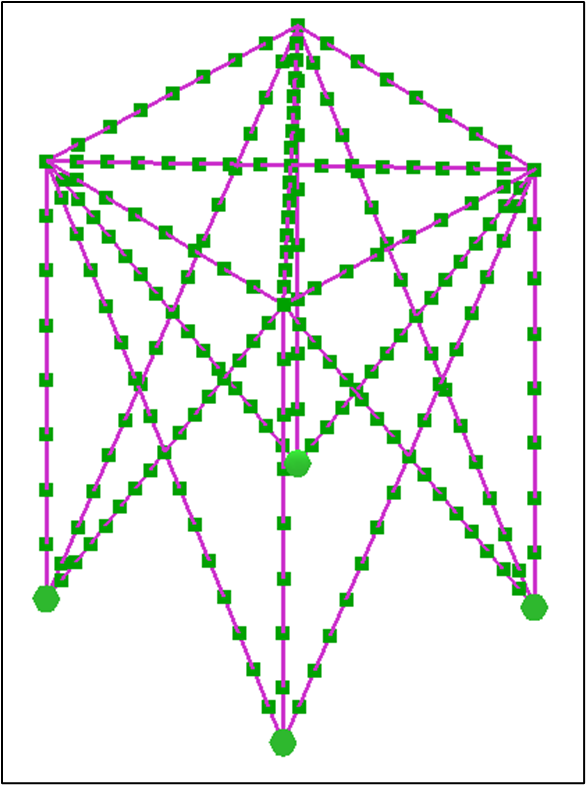Figure 4.29. Four node ports are created

• To constrain them, select four node ports created above → see the Property Tree and select (x, y, z, theta_x, theta_y, theta_z) in Constraint Type. The software will automatically do the same for other ports. After that, the black points will appear at four ports, it performs that four ports are constrained successfully.

Figure 4.30. Constraining node ports

Figure 4.31. The model with four constrained nodes

Step 7: Set Time Array & Time Steps

Figure 4.32. Model Set-up – Set Time Array & Time Steps

The incremental steps in pushover analysis represent the progression of loading from one limit state to another as the applied lateral forces increase. The magnitude of these increments depends on factors like the required accuracy, the complexity of the structure, and the specific objectives of the analysis. Smaller increments generally provide more precise results but lead to longer computation. In this step, we will guide you on how to set up time steps in Akselos Modeler for the load applied in the next step. 

• Time Array: The model has both constant loads and pushover loads, time_array should be an array with two entries: e.g. "time_array": "step_array([0.0, 1.5])*s". The solver initializes constant loads in the first step (at t = 0), and the pushover loads are added to the model in the second step.
  • To create a time array property, right-click on Model on the left pannel →Insert New→Generic Property →Property.

Figure 4.33. Inserting Model Property

• Rename the recently created property to time_array, and enter into the box as in the figure below.

Figure 4.34. Time array property

• Time Steps:
  • There are three child items in this property tree: load_substep_type, number_of_substeps, and time. The load_substep_type can be changed from a drop-down list of options, but the number_of_substeps must be given by the users. It should be noted that the time_array established previously is used to enter time.
  • There are three child items in this property tree: load_substep, number_of_substeps, and time.
  • The default value of max_arclen_substep is 100, which is sufficient in most cases. However, for some test cases, this value may need to be increased for the solver to trace a complete load-displacement curve.
  • The max_displacement_size stopping control method is optional, it uses the user input value as a criterion to stop solving. This input value represents the maximum allowable displacement (of any node in the structure) before the structure is considered collapsed.
  • To change the time steps settings, select default_time_stepping on the left panel.

Figure 4.35. Default_time_stepping

• In the Property Tree, right-click on default_time_step → Insert new → number_of_substeps (InPropertyArray).

Figure 4.36. Inserting number_of_substeps

• Change load_substep_type to ArcLengthContinuationProperties.

Figure 4.37. Setting load_substep_type

• Right-click on load_substep_type → Insert new → path_predictor_type (PathPredictorType).

Figure 4.38. Inserting path_predictor_type

• Right-click on auto_step_properties → Insert New → max_displacement_size (m).

Figure 4.39. Inserting max_displacement_size

• Right-click auto_step_properties → Insert New → max_substeps (PropertyArray).

Figure 4.40. Inserting max_substeps

• Change all values as in the figure below.

Figure 4.41. Setting default_time_stepping properties

Step 8: Apply Loads

Figure 4.42. Model Set-Up – Apply Loads

In this tutorial, there are three load cases applied to the mode (Self-Weight, Point-Load-Constant, Point-Load-Pushover). Self-Weight is applied on a subdomain selection and two Point-Load are applied on four nodes. To create a load applying on the node, we need to create Node Set and store them in Stored Selection.

• Create Node Set:
  • Change to the Collection ribbon → Show component tree → Right-click on Boundary Sets → Create Boundary Set → Node.

Figure 4.43. Creating Node Set

• Click on New Node → Select four nodes on top as the figure below.

Figure 4.44. Selecting four nodes for Node Set

• We need to turn on the PointLoad operator for this Node Set. Click on New Node → see the Property Tree and turn on PointLoad in Operators.

Figure 4.45. Turning on the PointLoad operator

•  After all, we need to save the change of component. Right-click on the component → Save Changes

Figure 4.46. Saving component

• Stored Selection for Self-Weight Load Case:
  • Change to the Model ribbon → On the left panel, right-click on Stored Selections → Create Subdomains Selection.

Figure 4.47. Creating Subdomains Selection

• Click on Subdomain Selection 1 → Select the model on the Graphic Window.

Figure 4.48. Storing Subdomain for Self-Weight load case

• Stored Selection for Point-Load Load Case:
  • Right-click on Stored Selections → Create Boundary Sets Selection.

Figure 4.49. Creating Boundary Set Selection

• Click on Subdomain Selection 1 → Select node-set (New Node created in the previous step) on the Graphic Window. Because the position of this node set coincides with another one, to select the right node-set, move the mouse to one of its nodes, use the Tab button to change to the right name shown at the bottom of the Graphic Window then click once.

Figure 4.50. Storing node sets for Point-Load load case

• Create Self-Weight Load Case:
  • Right-click on Load Cases → Create Load Case

Figure 4.51. Creating Load Case

• Right-click on Load Case 1 → Create Load

Figure 4.52. Creating load in load case

• Click on Load 1 → see the Property Tree and set them as in the figure below.

Figure 4.53. Defining Self-Weight load

Figure 4.54. The load vector of self-weight appeared after applying

• Create Point-Load-Constant Load Case:
  • Right-click on Load Cases → Create Load Case.

Figure 4.55. Creating Load Case

• Right-click on Load Case 2 → Create Load

Figure 4.56. Creating load in load case

• Click on Load 1 of Load Case 2 → see the Property Tree and set them as in the figure below.

Figure 4.57. Defining Point-Load

Figure 4.58. The load vectors of the point load (constant load) appeared after applying

• Create Point-Load-Pushover Load Case: We can copy from Load Case 2 and modify some values to use.
  • Right-click on Load Case 2 → Clone.

Figure 4.59. Creating load case by cloning from another one

• Expand Load Case 3 → click on Load 1 → Modify the values in the Property Tree as in the figure below.

Figure 4.60. Creating load in load case

To easily manage the load cases, we should rename them following the load (Right-click on it → Rename this Load Case or click on it → press F2 button)

• Load Case 1 = Self-Weight
• Load Case 2 = Point-Load-Constant
• Load Case 3 =Point-Load-Pushover

Figure 4.61. Renaming three load cases

Step 9: Create Solver Option

Figure 4.62. Solve – Create Solver Option

For the 1D beam element problem, we can only solve it with the FEA solver.

Figure 4.63. The default Solver Option

Figure 4.64. Setting FEA Solver

Figure 4.65. Adding some fields on Solver Option

Step 10: Create Scenario 

Figure 4.66. Solve – Create Scenario

Figure 4.67. Setting Scenario

• Set Solve List: Since there is only one scenario, select the default in Solve List to check that the default scenario is turned on.

Figure 4.68. Setting Solve list

Step 11: Sync Collection and Solve

Figure 4.69. Solve – Sync collection & Solve

Now you can proceed to solve the model. First, you have to save aks file to save all setting up the model → sync the collection to Akselos Dashboard → Run solving.

• Save aks File:
  • Click on the File tab →Save.

Figure 4.70. Saving aks file

• The Select destination to save the file window appears, enter the name into the File name box then click the Save button. You will receive a success message when the file is successfully saved.

Figure 4.71. Naming and saving aks file

• Sync Collection:
  • Change to the Collection ribbon → Click on Repository... → Sync.

Figure 4.72. Syncing collection

• Click the Commit button when this window appears.

Figure 4.73. Committing for synchronization

• Run Solving: Change to the Solutions ribbon → Click on the Solve button. The solving request will be submitted to Akselos Cloud. You will see the status of this request on the Solution tree. You can see the results once the solving is done, which is usually within seconds with Akselos solver. 

Figure 4.74. Solving model

Figure 4.75. Solution after solving.

5. Results

Figure 5.1. Validate – Compare with theoretical results.

After receiving the solution, you can study its solution fields.

See some related articles to get what you can do with the solution: ...

There are some solution fields (visualization & results). You can review it to compare it with yours.

Figure 5.2. Axial Force result

Figure 5.3. Displacement x-direction result

Figure 5.4. Displacement y-direction result

Figure 5.5. Displacement z-direction result

Figure 5.6. Plastic Indicator result

Figure 5.7. Shear Force results

Figure 5.8. Bending Moment results

• Validation:

The horizontal response calculated by the Akselos solver for the current jacket structure is compared to reference results [1] in the figure below. In terms of ultimate load capacity, the results appear to be in good agreement.

Figure 5.9. Load-displacement curves for the Four-legged jacket structure

[1] Engseth, A. Finite Element Collapse Analysis of Tubular Steel Offshore Structures, Div. of Marine Structures, The University of Trondheim, The Norwegian Institute of Technology, Trondheim, 1984.

• Before we start - Overview of Akselos simulation procedure
• Cantilever Beam with 1D Elements
• Cantilever Beam with 2D Shell Elements
• Cantilever Beam with Solid Elements