1. Introduction
1.1 What the Analytical Horizon Reports
The Coker Dashboard reports how many years each coke drum has before it reaches a limit set by a fitness-for-service standard. That figure is the Analytical Horizon, and it is the shortest of three results: Fatigue Life, Bulging Life and Crack Life. This article explains how Structural Performance Management for Cokers, written SPM for Cokers, computes each of the three, from the input data to the number that appears on the dashboard. Table 1 lists each result with the question it answers and the standard behind it.
Table 1. The results on the Coker Dashboard and the standard behind each
| Result | The question it answers | Standard | Section |
|---|---|---|---|
| Fatigue Life | How long until the accumulated fatigue damage at a location reaches 100 percent? | API 579-1/ASME FFS-1, 2021 edition, Part 14, Level 2, Method A | 3 |
| Bulging Life | How long until the plastic strain at a bulge reaches the local limit of the material? | API 579-1/ASME FFS-1, 2021 edition, Part 2, Annex 2D, Section 2D.3 | 4 |
| Crack Life | How long until a crack-like flaw grows to its critical size? | API 579-1/ASME FFS-1, 2021 edition, Part 9, Level 2 | 5 |
| Ovality | How far a cross-section is out of round, against the limit of the design code? | ASME BPVC Section VIII Division 1, paragraph UG-80 | 6 |
The Overall Coker Analytical Horizon panel on Home reports the shortest of the three lives, once for the pressurized and once for the non-pressurized components, and marks the assessment that sets it. Each assessment section below follows the same order: what the result means; the procedure, with its flowchart and steps, each step naming the clause of the standard it draws on; and where each result appears on the dashboard.
Info: For what each page displays and how to read it, see the Coker Dashboard article. This article covers how the numbers behind those pages are produced and leaves the equations to the standards it names.
1.2 How Plant Data Becomes a Result on the Coker Dashboard
Every result on the dashboard comes out of one process. Plant data and inspection data go in, a structural model of the drum turns them into stress, three assessments turn the stress into lives, and the lives go to the dashboard. Figure 1 shows the process.
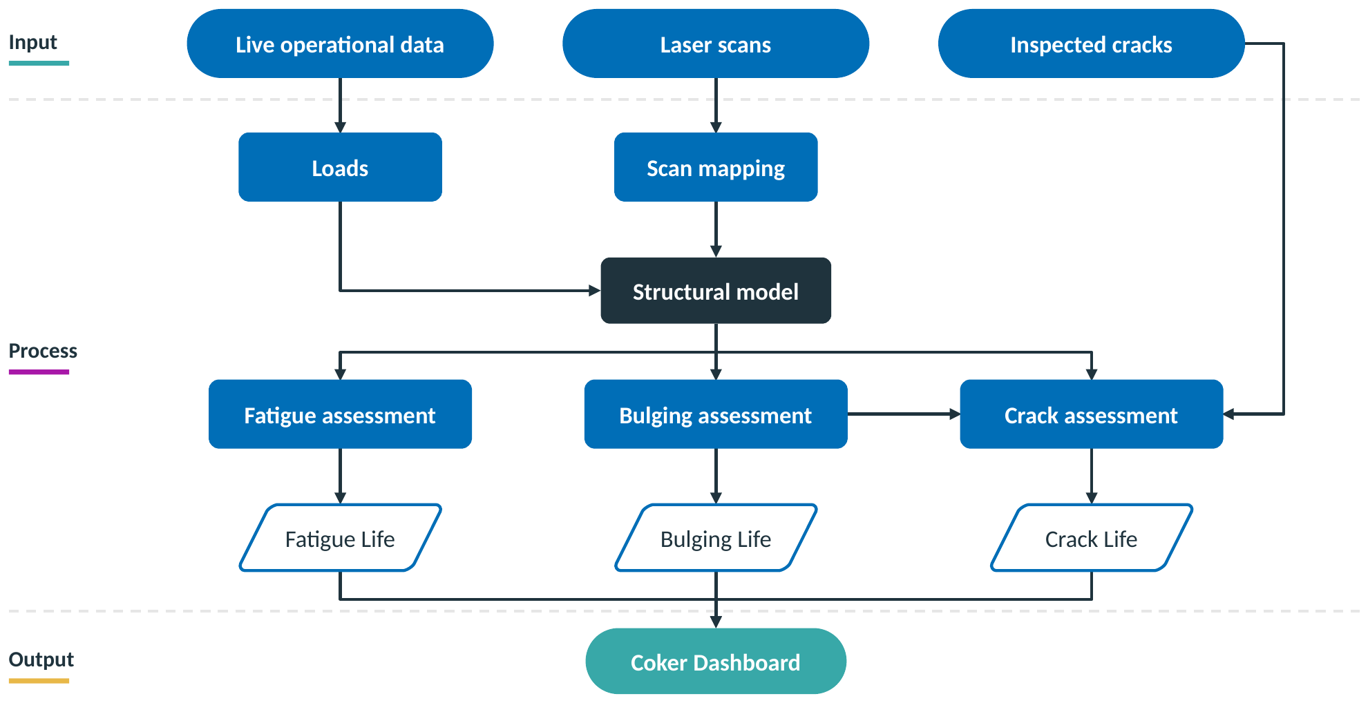
Figure 1. The assessment process, from plant data to the Coker Dashboard
Three inputs feed the process, and they arrive on two different schedules. Table 2 lists them.
Table 2. The three inputs to the assessment process
| Input | What it carries | When it arrives | Used by |
|---|---|---|---|
| Live operational data | Temperatures, pressures and liquid level recorded by the plant instruments | Every cycle | All three assessments and ovality |
| Laser scans | The measured shape of the inner wall of the drum | At each turnaround | Bulging and ovality, and crack through bulging |
| Inspected cracks | Inspection records the depth, length and position of each crack-like flaw. Where an inspection finds no crack, a reference flaw 1 mm deep and 100 mm long is assumed at each of the locations with the highest plastic strain limit fraction, written PSLF (Section 2.4). | At each turnaround | Crack |
The unit of time is one cycle: fill, coke, quench and decoke. For each processed cycle, the operational data becomes a set of loads on the structural model, and each assessment runs once on the result. The unit of place is one assessed location. Every result belongs to a location on the drum rather than to the drum as a whole, which is why the dashboard ranks locations.
The three assessments are linked. Bulging and crack both run on the model with the laser scan mapped onto it, and the locations where bulging is most severe are where the crack assessment places its reference flaws. Fatigue runs on the operational data alone.
1.3 Turnaround Results and Current Results
The bulging and crack assessments follow the turnarounds. Each turnaround supplies a new laser scan and a new set of inspected cracks, and the assessment of that data gives a fixed result for that turnaround. Bulging Inspection and Crack Inspection report these results one turnaround at a time.
From there the assessments carry on. The current result starts from the latest turnaround, applies the operating conditions of each new cycle, and advances the bulge and the crack size cycle by cycle. Crack Status, and the live entry in Inspection Data on Bulging Inspection, report the current result. Table 3 sets the two side by side for each assessment.
Table 3. Turnaround and current results for each assessment
| Result | Turnaround result | Current result |
|---|---|---|
| Fatigue Life | – | Fatigue Status, updated every cycle from the operational data |
| Bulging Life | Bulging Inspection, one entry in Inspection Data per turnaround | Bulging Inspection, the live entry in Inspection Data |
| Crack Life | Crack Inspection, one entry per turnaround that recorded a flaw | Crack Status |
Note: A turnaround result stays as it was assessed. A current result that moves between two cycles with no new inspection is responding to the operating conditions.
2. The Structural Model of the Coke Drum
All three assessments run on one structural model of the drum. The model takes the loads of each cycle and returns the stress at every assessed location. The laser scan gives it the measured shape of the inner wall that the bulging and crack assessments need.
2.1 What the Structural Model Represents
The structural model is a finite element model of the drum, built by Akselos engineers from its design geometry, its materials and its supports. It is divided into the zones printed in every ranked table on the dashboard. Table 4 lists what the model represents and how.
Table 4. What the structural model represents
| What is represented | How |
|---|---|
| Geometry | The design gives the elliptical head, shell, toriconical section and skirt of the drum. The laser scan adds the measured shape of the inner wall, as Section 2.3 describes. |
| Material | Properties are defined across temperature, because stiffness and strength fall as the steel heats. The temperature field of the cycle sets the property at each point. |
| Supports | The drum is restrained at the skirt and at the pipework connections. |
| Analysis type | The analysis is linear elastic for fatigue and elastic-plastic for bulging, where the strain beyond yield is the quantity being assessed. |
The model loaded with the operating data of a cycle is the as-is model. For bulging and crack, it is solved with the laser scan mapped onto the inner wall, so the bulges the drum has developed are in the geometry. In this article, as-designed means the drum as designed, with no operating load; no assessment runs on it.
2.2 Loads and Load Cases on the Model
Five loads act on the model, set by the recorded plant data and by the drum itself. Figure 2 shows how three recorded traces become loads on the drum. Table 5 lists all five and what sets each.
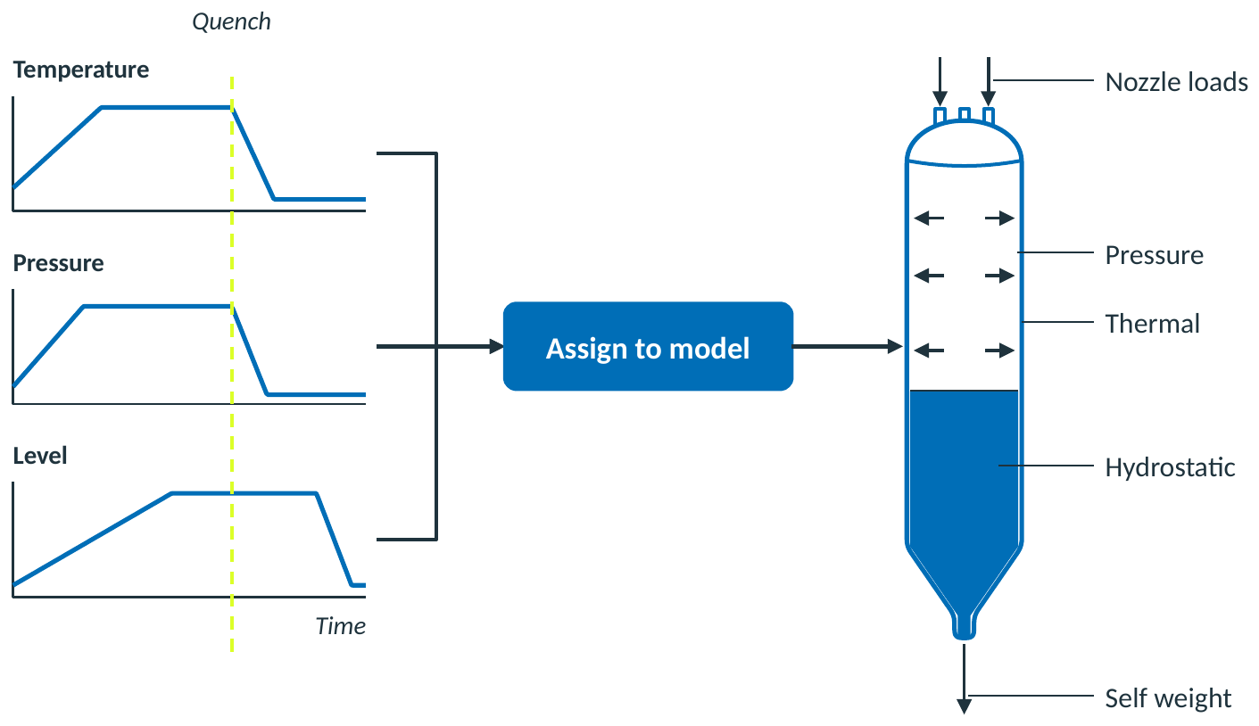
Figure 2. Recorded operating data assigned to the model as loads
Table 5. The loads on the model and what sets each
| Load | What sets it |
|---|---|
| Internal pressure | The recorded vessel pressure, acting on the whole containing surface |
| Hydrostatic pressure | The recorded liquid level, acting on the shell below it and growing with depth |
| Thermal load | The temperature field, interpolated between the thermocouple positions on the shell |
| Nozzle loads | The loads applied at the nozzles, which can account for the connected pipework and for pressure thrust |
| Self-weight | The weight of the vessel |
Pressure and level enter as two loads because they move differently through a cycle: pressure falls away during the quench while the drum is still full. The thermal load dominates. It is the gradient through and around the wall during the quench that loads the shell, so the interpolated field is kept within physical bounds between the instruments.
Before any of this, the record of each cycle is checked and repaired. A short gap is filled from the readings of the same instrument on either side of it, a failed instrument is replaced by a comparable one, or the record is rebuilt from neighboring instruments, in that order. A cycle with a gap longer than the configured limit is set aside and not assessed.
Each assessment applies the loads as its own load case, listed in Table 6.
Table 6. The load case of each assessment
| Assessment | Load case |
|---|---|
| Fatigue | The full loading history of the cycle: every recorded point from fill to decoke, solved in turn |
| Bulging | Load combination of the local failure check, per API 579 Annex 2D, Section 2D.3: internal pressure, hydrostatic pressure, self-weight and nozzle loads, multiplied by the load factor of the local criterion and by the remaining strength factor |
| Crack | The stress through the wall at the flaw location, and its maximum and minimum within the cycle, which set the range that drives growth |
2.3 How the Laser Scan Is Mapped onto the Model
The laser scan is turned into geometry the model can solve, so the bulges the drum has developed are present in the stress result. Figure 3 shows the three shapes involved.
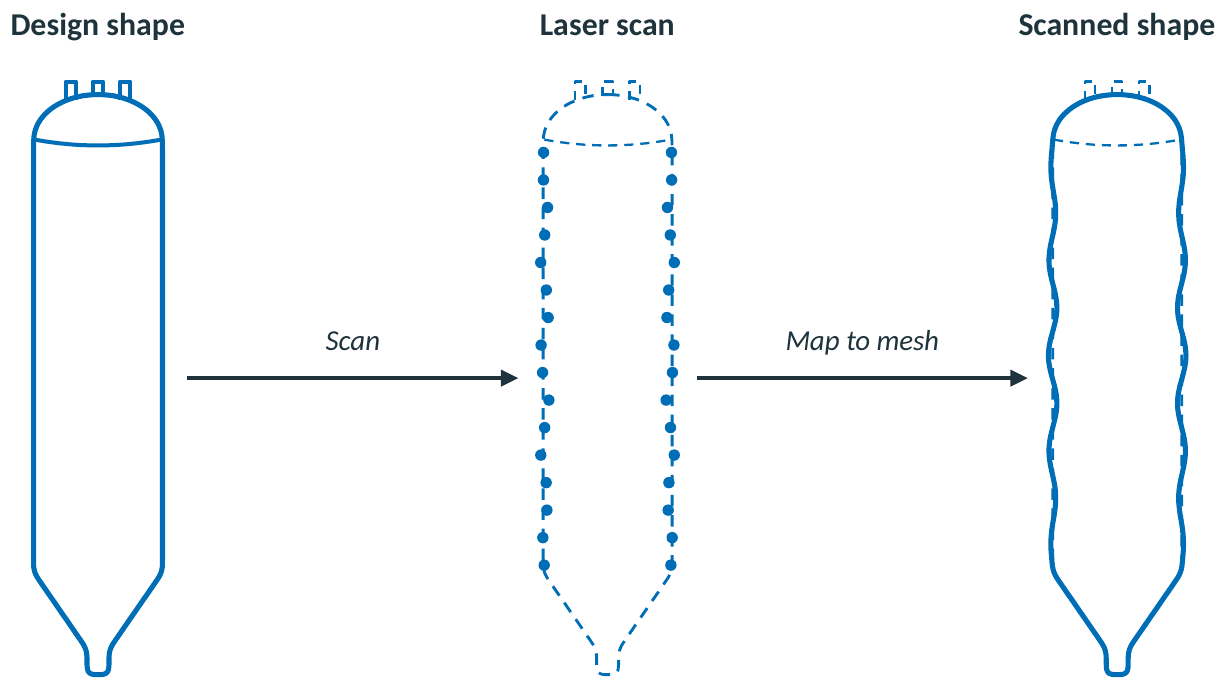
Figure 3. The design shape, the laser scan, and the scanned shape mapped onto the mesh
Five steps take the scan from the inspection files to a strain in the model:
- Read the scan. The inspection files give the inner radius at every angle and elevation the scan covers, converted to the units of the model.
- Clean it. Gaps and artifacts are either ignored or interpolated, from angle to angle or from elevation to elevation.
- Offset for the cladding. The drum is clad on the inside, so the cladding thickness is added to the scanned radius to reach the wall that carries the load.
- Map onto the mesh. The 360-degree point cloud at each elevation is interpolated onto the inner surface of the mesh, covering the elliptical head, the shell, the toriconical section and the upper skirt support. The mapping stays on the inner surface, because that is the surface the scan measures.
- Turn shape into strain. The mapping returns a field of permanent displacement. An initial displacement analysis imposes it on the model, with the temperature field of the quench setting the material properties, and returns the plastic strain the bulges represent as one equivalent plastic strain at each location.
That equivalent plastic strain is the link between the scan and the assessments. The bulging assessment measures it against a limit, and the crack assessment carries the stress it leaves behind as secondary stress.
Between turnarounds the bulge is predicted rather than measured. A machine learning model, written ML, is trained on the historical laser scans and predicts the inner radius ahead of the latest scan. A predicted bulge enters the model through the same mapping as a measured one.
2.4 How Cracks Enter the Assessment
A crack enters the assessment as a set of dimensions at a location on the model. The structural model supplies the stress at that location, and the crack assessment of API 579 Part 9 handles the flaw with the stress intensity and reference stress solutions the standard provides. Table 7 lists each input and its source.
Table 7. What the crack assessment needs and where it comes from
| What the assessment needs | Where it comes from |
|---|---|
| Crack depth and length | Inspection, or the reference flaw where no crack has been recorded |
| Location and component | Inspection: the elliptical head, shell, cone or skirt |
| Weld and post-weld heat treatment status | Whether the flaw sits in a weld, which selects the form of the growth law and brings in residual stress |
| Plane condition | Plane stress or plane strain at the crack front |
| Material properties | Yield strength, tensile strength and fracture toughness |
| Temperature | The temperature at the location, which sets the fracture toughness |
Where no crack has been recorded, the assessment still runs. Cracks are assumed to start at the locations with the highest PSLF from the bulging assessment. A reference flaw is placed at each of those locations as the worst case, with a depth of 1 mm, the depth API 579 gives for a reference flaw, and a length of 100 mm. Crack Status shows these two dimensions as Assumed Crack Depth and Bounding Crack Length. At the next inspection, a location where no crack is found is reset to this reference flaw.
A measured flaw is idealized before it is assessed. Its outline is replaced by a regular shape of one of the five flaw types in Part 9 (through-wall, surface, embedded, edge or corner), and a flaw lying at an angle is projected onto the plane of the maximum principal stress, per paragraph 9.3.6.
The stress at the flaw is then split by origin, because the standard treats each part differently. Primary stress comes from pressure. Secondary stress comes from the bulge, taken from the initial displacement analysis. Residual stress comes from welding, set by the weld geometry and thickness.
3. Fatigue Life Assessment
3.1 What Fatigue Life Means
Fatigue Life is the estimated service life left before the accumulated fatigue damage at a location reaches 100 percent, the failure threshold of API 579 Part 14, Level 2, Method A. It is expressed in operational cycles or in years.
Accumulated damage is a life fraction: the share of the location’s resistance to cyclic loading that the processed cycles have used. The calculation follows Part 14 at Level 2, Method A, an elastic stress analysis with equivalent stresses, and projects the damage rate forward to reach a life.
3.2 Fatigue Assessment Procedure
The fatigue assessment takes the live operational data from the plant instruments: temperatures, pressures and the other recorded process data. It follows API 579 Part 14, Level 2, Method A, with cycle counting per Annex 14C and the material stress-life curves, written S-N curves, of ASME BPVC Section VIII Division 2, Annex 3-F.
Info: The reference flowchart of the Part 14, Level 2, Method A procedure is in Coker Analytical Horizon Workflows Rev 1.2, Appendix A.
Figure 4 shows the procedure, which runs once for each processed cycle. The numbered badges match the steps below.
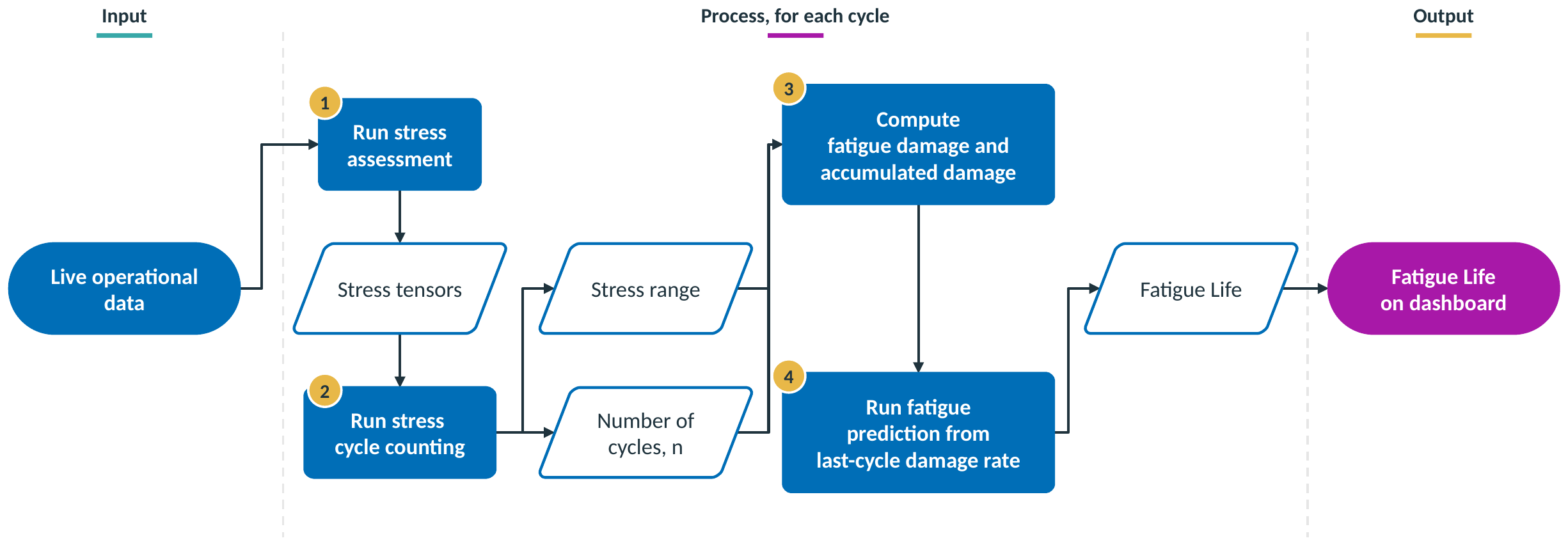
Figure 4. Fatigue Life assessment procedure
Step 1: Stress Assessment
A loading history is developed from the operational data of the cycle: pressure and temperature at each recorded point through fill, coke, quench and decoke. A linear elastic analysis of the structural model then gives the stress tensor at every assessed location for every point in that history.
Linear elastic analysis is the route Part 14 sets at Level 2, Method A, for stress that stays in the range where stress and strain are proportional. The result is a stress history at each location rather than one stress. The Stress tab of Result Viewer on Cycle Inspection shows this result as the von Mises stress at the most critical time of the cycle.
Step 2: Cycle Counting
The stress history of a cycle rises and falls many times, at different amplitudes, so it does not present a single stress range to assess. The cycle counting method of Annex 14C resolves it into a set of discrete stress ranges, each with its number of counted cycles, n.
Step 3: Damage Calculation
Each counted stress range is read against the material S-N curve of ASME BPVC Section VIII Division 2, Annex 3-F, which gives the allowable number of cycles, N, at that range. The damage of the cycle is the sum, over every counted range, of its counted cycles, n, as a share of its allowable cycles, N.
The damage of the cycle is added to the damage of every earlier processed cycle to give the accumulated fatigue damage. The accumulated figure only rises: a gentler cycle adds less, and nothing removes what has accumulated.
Step 4: Fatigue Life Prediction
The damage rate of the last cycle is projected forward until the accumulated damage reaches 100 percent. The cycles or years that projection takes are the Fatigue Life.
Because the rate comes from the last cycle, one severe cycle shortens Fatigue Life sharply and one mild cycle lengthens it, while the accumulated damage beside it moves only by the damage of that one cycle.
Figure 5 follows one location through the four steps, from the stress history of a cycle to the projected Fatigue Life. Panel 2 repeats the stress history of panel 1, and each arrow spans one counted stress range, from a peak to a valley.
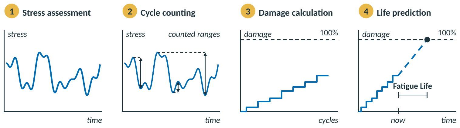
Figure 5. The four fatigue steps at one location
3.3 Where Fatigue Results Appear on the Coker Dashboard
Each step of the procedure that produces a reported result has a widget on the dashboard. Table 8 follows the steps in order.
Table 8. Fatigue steps, their outputs and where they appear
| Step | Output | Widget | Dashboard page |
|---|---|---|---|
| Stress assessment | Stress tensors at every location, through the cycle | Stress tab of Result Viewer: the von Mises stress | Cycle Inspection |
| Damage calculation | Damage of the cycle, and accumulated damage | Last Cycle Damage Max. Damage Top 10 Damage Locations, for pressurized and non-pressurized regions High Fatigue Damage Locations, for pressurized and non-pressurized regions Per-Cycle Damage Statistics Top 10 Best Cycles and Top 10 Worst Cycles | Fatigue Status |
| Total Single Fatigue Damage by Elevations | Cycle Inspection | ||
| Fatigue Life prediction | Fatigue Life | Min. Est. Fatigue Life Est. Fatigue Life at Pressurized Parts Est. Fatigue Life at Non-pressurized Parts Remaining Life [years] column of Top 10 Damage Locations Fatigue Life Prediction | Fatigue Status |
| Fatigue bar of Overall Coker Analytical Horizon | Home |
Fatigue Life is reported for the pressurized and the non-pressurized components separately, because the two groups carry different load histories. The junction where the skirt meets the shell is pressure-retaining and sits with the pressurized group.
4. Bulging Life Assessment
4.1 What Bulging Life Means
Bulging Life is the time from now until the plastic strain at a location reaches 100 percent of its local limiting strain, that is, until PSLF reaches 100 percent. PSLF is a life fraction for the local strain capacity of the material.
If the bulges keep developing as predicted, the location reaches the limit of the protection against local failure check of API 579 Annex 2D at the end of its Bulging Life. That is the point at which the material there has used its ductility.
Each new laser scan updates the bulge prediction, and with it the bulging results.
4.2 Bulging Assessment Procedure
The bulging assessment takes the historical laser scans and the live operational data. It follows the protection against local failure check of API 579 Part 2, Annex 2D, Section 2D.3.
Figure 6 shows the procedure. The ML model is built once from the historical laser scans, and the other steps run for each cycle. The numbered badges match the steps below.
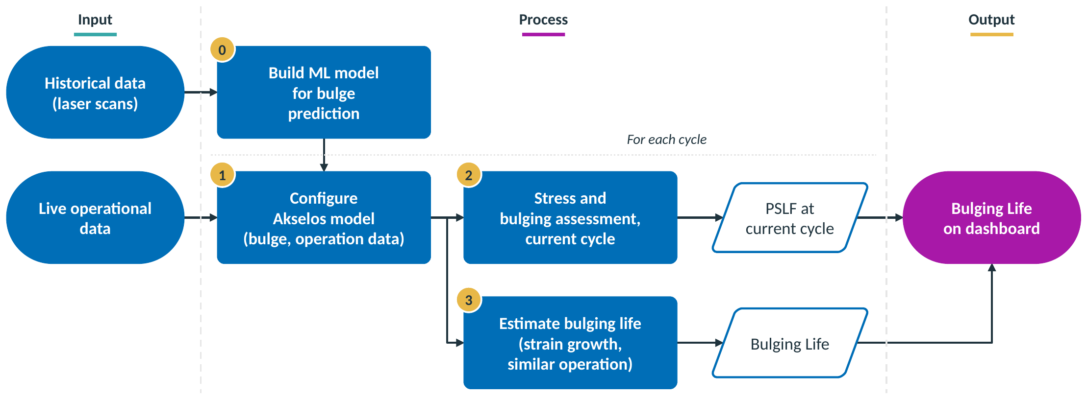
Figure 6. Bulging Life assessment procedure
Step 0: Build the ML Model
From the historical laser scans, an ML model is built to predict the bulge. It predicts the inner radius ahead of the latest scan, so the assessment can run on a bulge shape between turnarounds and into the future. Each new scan extends the record the model learns from.
Step 1: Model Configuration
The structural model is configured with the estimated bulge, mapped onto the inner wall as Section 2.3 describes, and with the operating data of the current cycle, such as the temperature field. The turnaround result uses the scan of that turnaround. The current result uses the bulge the ML model predicts for the cycle.
Step 2: Stress and Bulging Assessment
Two analyses run for the current cycle. The initial displacement analysis converts the bulge into the equivalent plastic strain it represents. An elastic-plastic analysis under the load combination of the local failure check then adds the strain of the operating loads, and returns the principal stresses and the von Mises equivalent stress at every location.
From that stress state, the limiting triaxial strain at each location is computed with the local strain limit of API 579 Annex 2D, which applies the elastic-plastic local strain limit of ASME BPVC Section VIII Division 2, paragraph 5.3.3, and its material factors. The limit falls as the stress becomes more triaxial, so it differs from location to location. The forming strain of the component is taken as zero, because the drum was heat treated after fabrication.
PSLF is the equivalent plastic strain, due to bulging and loading together, divided by the limiting triaxial strain, as a percentage. It is the quantity reported for the current cycle.
Note: The largest bulge is not necessarily the highest PSLF, because the limit changes with the stress state at each location. The PSLF at a location can also exceed 100 percent.
Step 3: Bulging Life Estimation
From the current strain growth, and with similar operating conditions assumed to continue, the bulging assessment is run again on the future bulges the ML model predicts. Bulging Life is the time until PSLF reaches 100 percent.
Running the assessment on the predicted shape, rather than extending the PSLF number, keeps the limit in step with the stress state as the bulge grows.
Figure 7 follows one location through the four steps, from the predicted bulge to the projected Bulging Life. In panel 0 the dots are the bulge measured at each turnaround and the dashed line is the ML prediction ahead of the latest scan. Panel 2 shows PSLF as the share of the location’s limiting strain that its plastic strain has used. In panel 3 the dashed line is the assessment re-run on the predicted bulges.
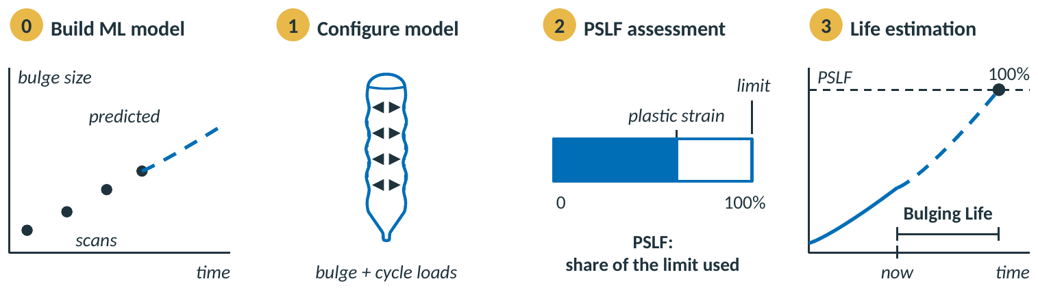
Figure 7. The four bulging steps at one location
4.3 Where Bulging Results Appear on the Coker Dashboard
All bulging results sit on Bulging Inspection, and the headline Bulging Life also reaches Home. Table 9 maps each step to its widget.
Table 9. Bulging steps, their outputs and where they appear
| Step | Output | Widget | Dashboard page |
|---|---|---|---|
| Model configuration | The as-is model with the estimated bulge and the operating data of the cycle | 2D Map of the Bulging of Inspection Visualization | Bulging Inspection |
| Stress and bulging assessment | PSLF at every location | Max. Plastic Strain Limit Fraction Top Severity Locations PSLF field of Inspection Visualization | Bulging Inspection |
| Bulging Life estimation | Bulging Life | Est. Bulging Life | Bulging Inspection |
Each turnaround entry in Inspection Data is the result of the assessment on that turnaround’s scan, and stays as it was. The live entry starts from the latest scan and runs on the operating data of each new cycle, with the bulge the ML model predicts.
Info: The likelihood classes on Top Severity Locations are a setting rather than part of the assessment. Their bounds are set by the asset owner’s subject-matter expert, and the Coker Dashboard article describes them.
5. Crack Life Assessment
5.1 What Crack Life Means
Crack Life is the estimated service time left for a detected or reference crack-like flaw to reach its critical size: the size at which its assessment point falls outside the Failure Assessment Diagram, written FAD, or at which the flaw penetrates the wall.
The calculation integrates subcritical crack growth by the Paris law with the operating stress of each cycle, following the flaw from its present size to that limit. Where no crack has been found, the flaw is the reference flaw at a highest-PSLF location, as Section 2.4 describes.
5.2 Crack Assessment Procedure
The crack assessment takes the inspected crack sizes and the live operational data. It follows API 579 Part 9, Level 2, with the Paris law per Annex 9F, Section 9F.5.2.2.
Info: The reference procedure of the Part 9, Level 2 assessment of crack-like flaws is in Coker Analytical Horizon Workflows Rev 1.2, Appendix B.
Figure 8 shows the procedure for one cycle, with the numbered badges matching the steps below. The loop from the estimated new crack size back to the current crack size carries the flaw into the next cycle.
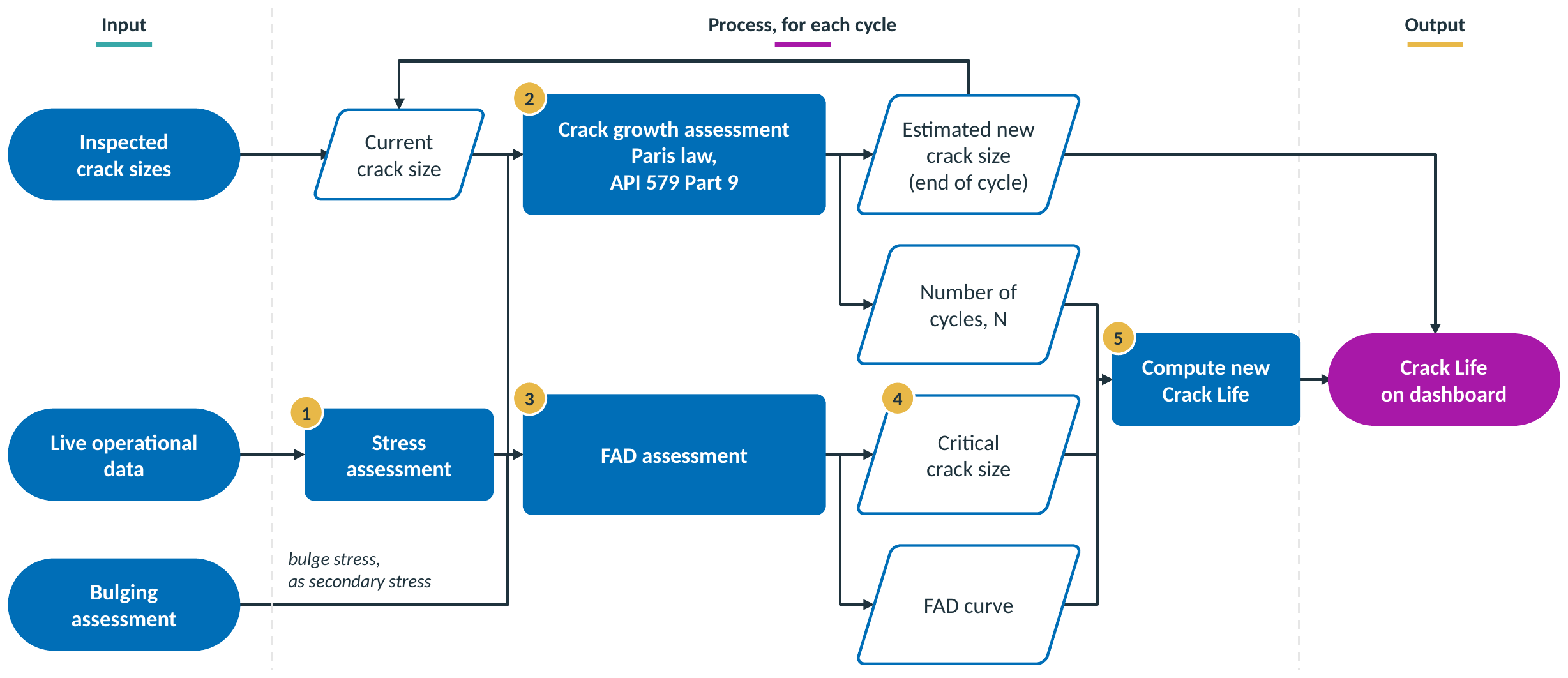
Figure 8. Crack Life assessment procedure
Step 1: Stress Assessment
The membrane and bending stresses at the flaw location are determined from the operational data: the stress through the wall, resolved into a part that is uniform across the thickness and a part that varies linearly across it. The load combinations are evaluated and the stress is classified per paragraph 9.3.4 into its primary, secondary and residual parts. The secondary part comes from the bulge: the bulging stress from the initial displacement analysis of the bulging assessment, shown as the bulging input in Figure 8.
The maximum and minimum stresses within the cycle are kept, because their difference sets the range that drives growth in the next step.
Step 2: Crack Growth Assessment
From the stress and the current crack size, which comes from inspection at first and is then updated each cycle, the Paris law of Annex 9F, Section 9F.5.2.2 gives the growth over the cycle and the new crack depth and length at its end.
The growth rate depends on the range of the stress intensity factor within the cycle, with the primary, secondary and residual contributions combined. The growth constants come from API 579 Table 9F.6, or Table 9F.6M in metric units, for the operating environment and temperature. A flaw in a weld uses the modified form of the law, which subtracts the threshold, and below the threshold the flaw does not grow.
Growth is computed in small increments. An increment is accepted only if the crack size and the stress intensity range each change by less than a set tolerance; otherwise it is reduced and computed again. The number of cycles, N, is counted as the flaw grows.
Step 3: FAD Assessment
The new crack size and the membrane and bending stresses are checked on the FAD, together with the material properties. Four quantities place the point:
- Yield and tensile strength, from material test data or from the nominal values of the material specification.
- Fracture toughness, from Annex 9F: the lower of the lower-bound toughness curve at the metal temperature and the upper-shelf value.
- The load ratio: the primary reference stress, from the reference stress solutions of Annex 9C, divided by the yield strength.
- The toughness ratio: the primary stress intensity plus the secondary and residual stress intensity, with the secondary and residual part corrected by the plasticity interaction factor of API 579 Table 9.3, divided by the fracture toughness. The stress intensity solutions come from Annex 9B.
The flaw is acceptable when the point lies inside the FAD envelope and the load ratio is below the cut-off the material sets.
The diagram judges a flaw against two failure modes at once: fracture, when the material at the crack tip lacks the toughness to stop the crack from extending, and plastic collapse, when the remaining section gives way. The toughness ratio measures the first and the load ratio the second.
Step 4: Critical Crack Size
The critical crack size is the size at which the assessment point moves outside the FAD, or the crack becomes through-wall, for the fracture toughness of the material and the current loading. It is found by stepping the crack size up from its current value toward a theoretical upper bound set by the geometry, with the FAD checked at each step. The last size inside the envelope is the critical size.
Step 5: Crack Life Estimation
The crack growth of the current cycle is projected forward until the crack reaches the critical size. The cycles that projection takes, converted to time, are the Crack Life.
The crack size carried into the next cycle comes from the growth computed in this one, so Crack Life moves as the flaw grows as well as with the operating data.
Figure 9 follows one flaw through the five steps. Panel 1 is a section through the wall at the flaw, with the inner wall on the left and the outer wall on the right; the wavy edges mark where the piece is cut from the rest of the wall. The crack is a surface flaw that starts at the inner wall. The arrows are the stress that pulls the crack open; their length changes across the wall thickness, and Step 1 resolves that change into membrane and bending parts.
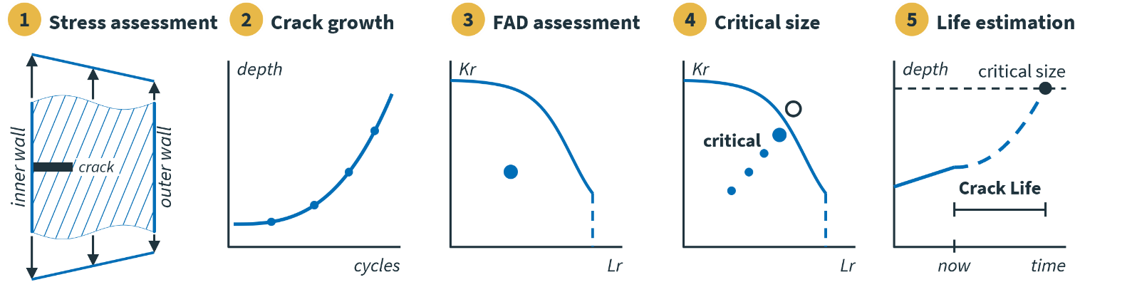
Figure 9. The five crack steps for one flaw
5.3 Where Crack Results Appear on the Coker Dashboard
Crack Status carries the current result and Crack Inspection the result of each turnaround that recorded a flaw. Table 10 maps each step to its widget.
Table 10. Crack steps, their outputs and where they appear
| Step | Output | Widget | Dashboard page |
|---|---|---|---|
| FAD | Load ratio, toughness ratio, and the result against the envelope | Lr, Kr and Status columns of Crack Details FAD Curve: API 579 Part 9 Level 2 | Crack Status and Crack Inspection |
| Crack Life estimation | Crack Life | Minimum Estimated Crack Life: the shortest current Crack Life on the drum, with its flaw and zone Estimated Crack Life [years] column of Crack Details: the current Crack Life of every tracked flaw, measured or reference, for the cycle selected in Cycle ID | Crack Status |
| Estimated Crack Life [years] column of Crack Details: the Crack Life of each flaw that turnaround recorded, at its measured size, against the cycle in the Cycle ID column | Crack Inspection | ||
| Crack bar of Overall Coker Analytical Horizon | Home |
The two Estimated Crack Life [years] columns answer different questions. On Crack Status the value is current: each tracked flaw starts from the latest turnaround, measured or reference, and is grown through every processed cycle since, so the value moves with each new cycle. On Crack Inspection the value is a record of one turnaround: each flaw is assessed once, at the size that turnaround measured, and the value stays as it was.
Note: The same flaw can show a different life on the two pages. The inspection value belongs to the day of the turnaround, and the status value to the selected cycle, including the growth since that turnaround.
6. Ovality Assessment
6.1 What Ovality Measures
Ovality is how far a cross-section of the drum is out of round. The ovality assessment monitors it at the elevations of the shell wall and at the flange of the drum. It is a shape check rather than a life: each result is checked against the out-of-roundness limit of ASME BPVC Section VIII Division 1, paragraph UG-80, under which the difference between the largest and the smallest inside diameter at any cross-section shall not exceed 1 percent of the nominal diameter there. Figure 10 shows the two diameters the check compares.
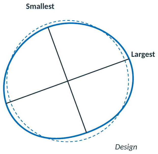
Figure 10. The largest and smallest inside diameter at one elevation
At each elevation the radius is taken at every degree around the circumference. Each diameter is the sum of two radii at opposite angles, which gives 180 diameters per elevation, so a wall that has moved out on one side reads as off-center rather than larger. The nominal diameter is the mean of the 180. Ovality is the largest diameter minus the smallest, divided by the nominal, as a percentage.
6.2 Ovality Assessment Procedure
The ovality assessment takes the historical laser scans and the live operational data. The shell wall is checked on the inspection data. The flange, which the laser scan does not cover, is checked on the structural model, configured as in the bulging assessment.
Figure 11 shows the procedure. The numbered badges match the steps below.
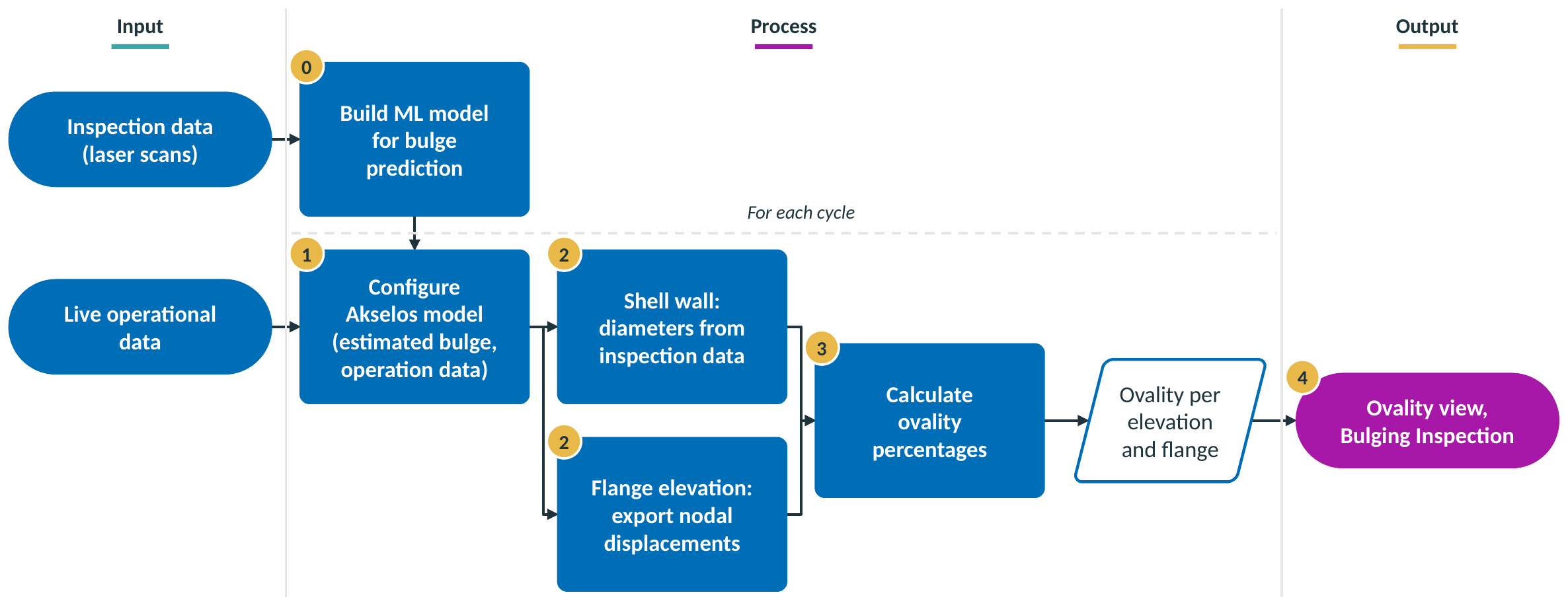
Figure 11. Ovality assessment procedure
Step 0: Build the ML Model
The ML model for bulge prediction is built once from the historical laser scans. It is the model of Step 0 in Section 4.2.
Step 1: Model Configuration
The structural model is configured with the bulge the ML model estimates, mapped onto the inner wall as Section 2.3 describes, and with the operational data of the cycle.
Step 2: Ovality Projection
The diameters come from two sources, because the laser scan does not cover the flange:
- For the shell wall, the inspection data at each elevation.
- For the flange elevation, the nodal displacements of the model at the time step of the cycle when the maximum von Mises stress occurs.
Step 3: Ovality Percentage Calculation
The ovality percentage at each shell elevation and at the flange is calculated from the inspection data and the flange displacements. Each percentage is the largest diameter minus the smallest, divided by the nominal diameter, as Section 6.1 describes.
Step 4: Monitoring
The results are shown in the Ovality view on Bulging Inspection, where values at or above 1 percent, the limit of paragraph UG-80, are highlighted for further review.
6.3 Where Ovality Results Appear on the Coker Dashboard
The ovality results appear in the Ovality view of Bulging Inspection Results on Bulging Inspection. Table 11 maps each step to its widget.
Table 11. Ovality steps, their outputs and where they appear
| Step | Output | Widget | Dashboard page |
|---|---|---|---|
| Ovality projection | Inner diameters around each shell elevation | Ovality view of Bulging Inspection Results: the polar cross-section of the elevation chosen | Bulging Inspection |
| Ovality percentage calculation | Largest and smallest inner diameter and ovality percentage at each elevation | Selected Elevation Ovality Information: the maximum and minimum inner diameter and the ovality percentage of the elevation chosen Maximum Ovality Information: the highest ovality percentage on the vessel and the elevation it occurs at | Bulging Inspection |
| Monitoring | Ovality at or above 1 percent, highlighted | Ovality percentages at or above 1 percent, highlighted in orange | Bulging Inspection |
Nothing accumulates and no life is projected, so ovality is not part of the Analytical Horizon.
7. Standards, Sources and Related Articles
7.1 Standards Used
Table 12 lists the standards and editions this article cites.
Table 12. Standards used in this article
| Standard | Designation | Edition | Used for |
|---|---|---|---|
| Fitness-For-Service | API 579-1/ASME FFS-1 | 2021 | Part 14, Level 2, Method A, for fatigue Part 2, Annex 2D, Section 2D.3, for the local failure check in the bulging assessment Part 9, Level 2, with Annexes 9B, 9C and 9F, for crack-like flaws |
| Rules for Construction of Pressure Vessels, Alternative Rules | ASME BPVC Section VIII Division 2 | 2019 | Annex 3-F, for the S-N curves Paragraph 5.3.3, for the local strain limit that API 579 Annex 2D applies |
| Rules for Construction of Pressure Vessels | ASME BPVC Section VIII Division 1 | – | Paragraph UG-80, for out-of-roundness |
The step-by-step procedures behind Part 14, Level 2, Method A and Part 9, Level 2 are shown in Coker Analytical Horizon Workflows Rev 1.2: Appendix A for fatigue and Appendix B for crack-like flaws.
7.2 Related Articles
- The Coker Dashboard article: every page and widget named above, and how to read it.
- Fatigue Use Cases on the Coker Dashboard: two fatigue use cases, page by page.