1. Introduction
Floating Offshore Wind Turbines (FOWTs) are renewable energy assets secured on floating foundations designed to harness offshore wind energy. The floating base configuration allows for deployment in deeper water regions where wind resources are stronger and more consistent due to a lack of physical obstacles.

Figure 1.1 Floating Offshore Structure
This article describes the setup and application of an Akselos Structural Twin model for a Floating Offshore Wind Turbine based on the DeepCwind reference configuration. The purpose is to document how the structural model is defined, how external hydrodynamic and aerodynamic loads are transferred into the Structural Twin, and how the model is used to evaluate global and local structural response under operational and environmental loading.
The content is intended for engineers configuring or reviewing Floating Offshore Wind Turbine models in Akselos Modeler, particularly in workflows that couple structural analysis with results from external hydrodynamic simulation tools.
The Floating Offshore Wind Turbine is represented using a reduced order Structural Twin derived from a detailed finite element model. The model captures the global stiffness, mass distribution, and primary load paths of the floating substructure and tower while enabling efficient evaluation across multiple load cases.
2. Structural Twin Model Specification
Before moving into the model specification details:
- A sample model for the Floating Offshore Wind Turbine is available in the standard sample collection. This sample can be used as a reference for model setup, load organization, and result review within SPM.
- The workflow and examples described in the following sections are demonstrated using Akselos Modeler 2025.10.
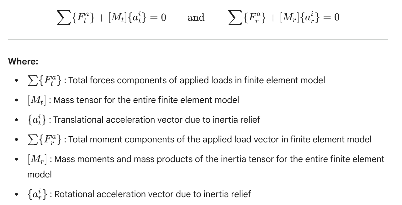
2.1. Model summary
The structural twin of the DeepCwind unit is architected to represent the floating foundation of the semi-submersible wind turbine. The simulation model specifically targets the floater foundation to capture its structural response under hydrodynamic and operational loads.
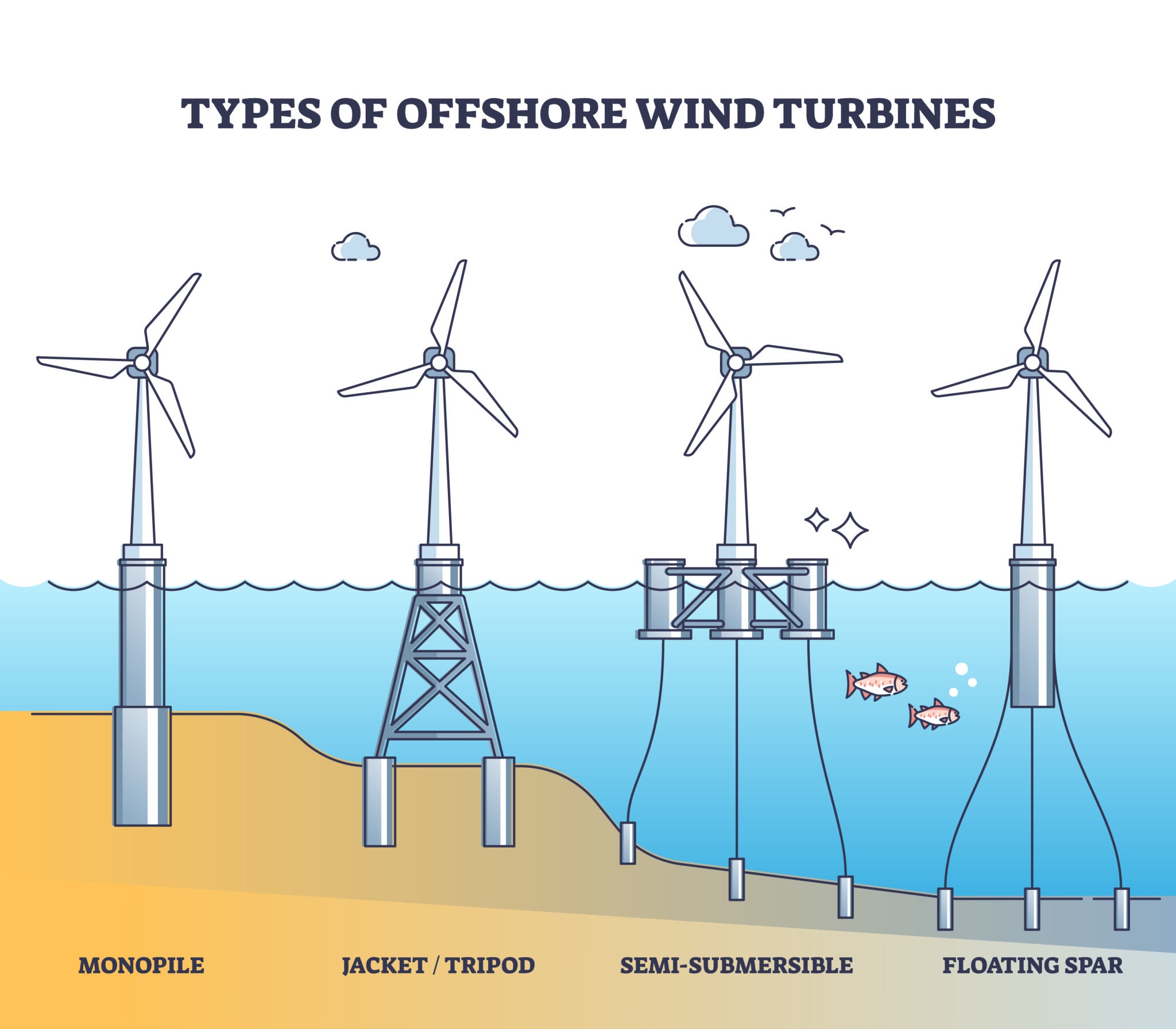
Figure 2.1 Types of Offshore Wind Turbine
The geometry is discretized into specialized subdomains to optimize the balance between computational speed and mechanical fidelity.

Figure 2.2 Floating Offshore Wind Turbine foundation model
System Scale: The model contains approximately 1.86 million degrees of freedom (DoF), ensuring detailed capture of stress and strain gradients across the asset.
Element Discretization: The geometry is meshed using a hybrid approach to best represent different structural members:
Pontoon System: Modeled using Shell elements to capture membrane and bending behavior in the base structure.
Columns: Modeled using Shell elements reinforced with 1D stiffeners. This allows for precise representation of the stiffened cylindrical structures without the excessive computational cost of modeling every stiffener as 2D plates.
Mooring Connections: Modeled using 1D beam elements configured as 6-DoF spring connectors at the three mooring lines, simulating the elastic boundary interface between the floater and the anchoring system.
2.1. Material and Thickness
The structural twin utilizes Elasticity Isotropic Material definitions to replicate the mechanical behavior of the DeepCwind foundation. To accurately represent the physical mass of the asset, including ballast and secondary components, without modeling every internal detail, the material density is scaled across specific subdomains while maintaining standard steel stiffness parameters. 1D stiffener elements automatically inherit the material properties of the Shell subdomain to which they are attached.
| Parameter | Value / Range | Description |
|---|---|---|
| Material Type | Elasticity Isotropic Material | Standard linear elastic behavior. |
| Young's Modulus | 215 GPa | Stiffness modulus for the steel structure. |
| Poisson's Ratio | 0.3 | Transverse deformation ratio. |
| Mass Density | 1,834 to 86,100 kg/m³ | Variable density scaled to match the physical weight distribution of the floater and ballast. |
Material is applied in Subdomain, users can select Subdomain(s) and view the material properties on the Properties Tree or Show Property tool to check the material parameters of the whole model.
How to view any subdomain materials properties
STEP 1: Change Selection Mode (top right of graphic window) to Subdomains → Click on a Subdomain on Graphic window
STEP 2: On the Property Tree (bottom left) → Expand the material → view properties

Figure 2.3 View Material parameters via Properties Tree
How to view all component materials properties:
STEP 1: Change Selection Mode (top right of graphic window) to Subdomains → Expand the Property → Select Load more… → Wait a moment for the assets to be loaded in

Figure 2.4 Load More… to enable more fields
STEP 2: Expand the Property → Select a material property field → view the property of the whole model subdomains

Figure 2.5 Select a field to visualize
The selected property (mass_density) belongs to ElasticityMaterialBeam properties, so the visualization will be the mass_density of all the beams as below.

Figure 2.6 View mass_density of beams via Show properties tool
For shell subdomains, the mass_density belongs to ElasticityMaterialShell, as shown in the figure below:

Figure 2.7 mass_density of ElasticityMaterialShell
2.2. Boundary Conditions
To simulate the unconstrained, free-floating behavior of the semi-submersible foundation, the structural twin utilizes Inertia Relief as its primary boundary condition. In this approach, the simulation treats each time step as quasi-static, where any residual forces from applied loads are instantly counteracted by inertial forces generated through an equivalent acceleration field. This method ensures global equilibrium is maintained throughout the analysis without imposing artificial kinematic constraints that would otherwise alter the physical response of the floating asset.
The equilibrium is mathematically enforced at every time step using the following governing equations:
2.3. Applying Loads
The structural twin operates by integrating external environmental and operational data to drive the mechanical simulation. External loads are applied to the floater structures based on the outputs of coupled model analyses (e.g., OrcaFlex and OrcaWave). The forces are computed in the time domain, where a reduced-basis finite element analysis (RB-FEA) static simulation is performed at each step of the time series to determine the structural response.
2.3.1. Load Mechanism
The structural twin operates on a rigorous data transfer pipeline that integrates frequency-domain hydrodynamics and time-domain operational physics into the RB-FEA environment. This framework synthesizes outputs from specialized solvers to ensure the structural analysis is driven by accurate, physics-based boundary conditions. The integration bridges the gap between the Potential Flow Model (frequency domain) and the Aero-Elasto-Servo-Hydro Model (time domain) through automated API scripts that convert solver outputs (e.g., .sim, .owr) into compatible .npz data bundles for the structural twin.
The integration process is executed through three distinct workflows, each handling specific data streams:
Load Transfer Workflow: Establishes the high-level architecture connecting the potential flow solver, the coupled dynamic solver, and the structural twin.
OrcaFlex Data Transfer: Manages the extraction of time-domain operational data, including vessel motion and connection loads.
OrcaWave Data Transfer: Handles the spatial mapping of frequency-domain hydrodynamic pressures onto the structural mesh.
Load Transfer Workflow
The workflow coordinates three simulation domains to ensure high-fidelity stress analysis:

Figure 2.8 Akselos’ floating offshore wind load transfer workflow
Frequency Domain (Potential Flow): Hydrodynamic databases (added mass, damping, wave load RAOs) are generated in solvers like OrcaWave.
Time Domain (Aero-Elasto-Servo-Hydro): Global performance and motion are simulated in OrcaFlex, incorporating wind, waves, and control systems.
- Structural Twin (RB-FEA): The Akselos model ingests the outputs from both domains. Crucially, the hydrodynamic database is interpolated directly onto the Akselos mesh, allowing for precise pressure mapping rather than simplified load application.
OrcaFlex to Akselos Data Transfer
This pipeline handles Time Domain data. An automated API script extracts simulation results from the coupled model (.sim file) and converts them into a compatible .npz time-series bundle.

Figure 2.9 OrcaFlex to Akselos Data Transfer
The following outputs are extracted from the coupled model and used as inputs to the structural analysis for each load case:
Vessel Dynamics: Time series of the six (6) DoF foundation positions, velocity, and acceleration.
Connection Loads:
Time series of the mooring tension loads.
Time series of the tower base forces and moments.
Environment & Wave Kinematics:
Wave Components: Frequency, amplitude, phase, and wavelength of the irregular wave.
Wave Data: Wave headings.
Current: Current speed profile and direction.
Coefficients: Drag and added mass coefficients of each member for both Morison elements of the floater type and 6D buoys from the OrcaFlex model.
OrcaWave to Akselos Data Transfer
This pipeline handles Frequency Domain data. The API script processes the OrcaWave output file (.owr) to extract the hydrodynamic pressure database. A spatial Interpolation process is performed to map the pressure data from the potential flow panels directly onto the structural twin's finite element mesh.

Figure 2.10 OrcaWave to Akselos Data Transfer
Hydrodynamics: Hydrodynamic pressure database, in the frequency domain, from OrcaWave (diffraction and radiation pressures).
Geometry: Mesh (or panel geometry) used in OrcaWave for the potential flow model.
Wave Parameters: Wave Headings and Wave Frequencies.
In Akselos Modeler, the corresponding loads are listed as below:
| Load Name | Mechanism | Akselos Load Type | DeepCwind | Load Parameters |
|---|---|---|---|---|
| Gravity (self-weight) and ballast weight | The structure is divided into multiple subdomains in Akselos Modeler, each assigned a material density. The self-weight of the structure is computed from these densities and included in the global mass matrix. Ballast weights are represented either by locally increasing the material density or by applying equivalent point loads distributed to surrounding shell elements. The total mass contribution, including ballast, is included in the mass matrix used by OrcaFlex during the coupled simulation. | Material Volume Load |  | Local gravity vector in x, y, z (m/s²) |
| Hydrostatic pressure | Hydrostatic pressure, including static buoyancy and hydrostatic restoring forces, is computed in Akselos on each element of the outer surface of the floating structure. The pressure is evaluated based on sea water density, gravity, and the instantaneous position of the structure at each simulation time step, using rigid-body motions extracted from OrcaFlex. A constant water level is assumed throughout the simulation, and hydrostatic pressure variations caused by wave elevation are not applied. This approach is consistent with the hydrostatic formulation used for vessel objects in OrcaFlex.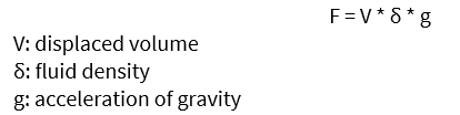 | Floater Hydrostatic Load Pressure |  | Centre of rotation (m)Sea density (kg/m³)Gravity constant (g)Sea water level (m)Body motion (heave, roll, pitch, yaw) |
| Hydrodynamic diffraction and radiation loads | Diffraction and radiation pressure transfer functions are computed in OrcaWave using frequency-domain potential flow analysis. These frequency-dependent pressures are stored in the Akselos model and applied as distributed normal loads on the external surfaces of the floating structure. During the simulation, the pressures are reconstructed in the time domain using motion and wave information to ensure consistency with the coupled OrcaFlex response. | Normal Load |  | Frequency pressure contained in the Akselos model (Hz)Time step coefficient (-) |
| Morison drag and inertia loads | Hydrodynamic forces on slender structural members are computed in OrcaFlex using Morison theory. These forces include drag components related to relative fluid velocity and inertia components related to fluid acceleration. The resulting forces are transferred to Akselos Modeler and applied as distributed wave loads consistent with the kinematics used in the coupled simulation.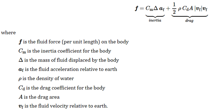 | Wave Load |  | Morison element properties: drag diameter (m), drag coefficient (-) Body kinematics data Current data Wave components Kinematic stretching data Seabed (m) Water depth (m) Water density (kg/m³) Wave heading (deg) |
| Mooring line forces | Mooring line tensions are computed in OrcaFlex during the coupled time-domain simulation. These tensions are extracted and applied in Akselos Modeler as concentrated point loads at the corresponding mooring attachment locations on the floating structure.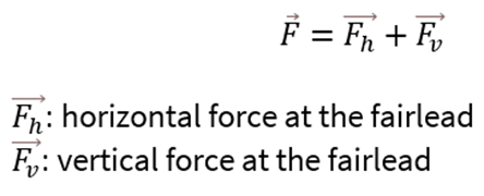 | Point Load |  | Mooring line tension (N)Attachment location (m) |
| Tower base loads | Forces and moments transmitted from the wind turbine tower to the floating substructure are computed in OrcaFlex as part of the coupled aero-hydro-servo-elastic analysis. These loads are applied in Akselos Modeler at the tower base interface to represent the interaction between the tower and the floater. | Point Load |  | Force components (N)Moment components (N·m) |
| Rigid-body translational acceleration | Rigid-body translational and rotational accelerations of the floating structure are extracted from OrcaFlex and applied in Akselos Modeler as inertial loads. Translational accelerations generate equivalent volume forces, while rotational accelerations generate inertial moments, ensuring consistency with the coupled dynamic response. | Material Volume Load Material Rotary Acceleration |  | Translational acceleration in x, y, z (m/s²) |
Load Application Workflow
To effectively implement these loads within the structural twin environment, specific preparatory configurations are required. Before load cases can be defined, the model must be organized to recognize where forces are applied and how external data is ingested. This involves defining:
- Create Stored Selections (define group of entities that is under the same load)
- NPZ Bundle (read .npz file from OrcaFlex)
- Model variables (manage properties that used for applying loads and fatigue analysis setting up)

Figure 2.11 Input for Loads
The subsequent sections provide a comprehensive breakdown of these steps, detailing how to configure Stored Selections for entity management, utilize NPZ Bundles for data import, and define Model Variables for efficient property mapping.
2.3.2. Entity Management (Stored Selections)
To facilitate precise load application and efficient model management, the structural twin utilizes Stored Selections. These are user-defined collections of geometric entities, such as components, subdomains, boundary sets, or element sets, that are saved within the model file (.aks) and referenced by name during the setup of loads and analyses.
Users can explore and modify these selections via the Object Tree, where they are categorized by type.

Figure 2.12 Four Stored Selection types
- Component selections: Allow storage of one or multiple complete components.
- Subdomains selections: Allow storage of one or multiple subdomains that belong to one or multiple components.
- Boundary Sets selections: Allow storage of one or multiple surfaces, nodes, or edges on which boundary conditions or loads can be applied; they can belong to one or multiple components.
- Element Sets selections: Allow selection of one or multiple elements that belong to one or multiple components.
To view object(s) in a Stored Selection:
On Structure Tree → Expand the Model → Expand the Stored Selections → Select a Stored Selection and View the visualization on Graphic Window.
Figure 2.13 Stored Selections of DeepCwind 5 MW model
The DeepCwind model configuration relies on three primary categories of stored selections:
Boundary Sets Selection:
- Mooring_1: a node in component 5 MW_BC2_Bottom that is used to apply a Point Load representing the mooring force
- Mooring_2: a node in component 5 MW_BC1_Bottom that is used to apply a Point Load representing the mooring force
- Mooring_3: a node in component 5 MW_BC3_Bottom that is used to apply a Point Load representing the mooring force

Figure 2.14 Stored Selection of Mooring
- Tower: a node in component 5 MW_MC_Top that will be used to apply Point Load, which represents a force in the tower

Figure 2.15 Stored Selection of Tower
- Hydrostatic: 24 surfaces that will be applied Hydrostatic Load

Figure 2.16 Stored Selection of Hydrostatic
- Wetted_panels: 14 surfaces that will be applied Diffraction Load and Radiation Load

Figure 2.17 Stored Selection of Wetted_panels
- Morison: 134 surfaces that will be applied Wave Load

Figure 2.18 Stored Selection of Morison
Subdomains Selection:
- Self_weight: 137 subdomains that will be applied Self Weight Load and Acceleration Load

Figure 2.19 Stored Selection of Self_weight
Components Selection:
- Fatigue Components: components that will be used to calculate fatigue damage

Figure 2.20 Stored Selection of Fatigue Components
2.3.3. NPZ Bundle
The structural twin leverages the NPZ Bundle tool to ingest external simulation data stored in .npz files. This approach is essential for the DeepCwind model, as the majority of environmental and operational loads are derived from external solvers (e.g., OrcaFlex) rather than being defined natively within the structural model file (.aks).
The tool categorizes imported data into two distinct property types:
npz_coeffs: Stores static coefficients that remain constant throughout the analysis.
npz_time_series: Stores dynamic coefficients that vary with each simulation time step.
To view the NPZ Bundle:
On Model Tree → Expand the NPZ Bundle
Figure 2.21 NPZ Bundle is located on the Model Tree
Select npz_coeffs or npz_time_series → On Property Tree (left bottom) → Click on a property in files → See the values/properties on the Table & Chart 
Figure 2.22 npz_time_series properties
To manage the temporal resolution of the simulation, the npz_time_series property includes a filter function that allows users to define specific time steps for analysis:
Slide: Selects a continuous range of steps defined by a
start_indexandend_index, applying a specificstrideinterval.ExcludeSome: Includes all time steps except those explicitly listed for exclusion.
IncludeOnly: Restricts the analysis to a specific list of time steps.
2.3.4. Model Variables
Model Variables serve as the internal data management layer within the structural twin. Located in the Model tab, these variables store dynamic properties and environmental parameters imported from external sources (such as the NPZ bundles).
Rather than referencing external data files directly within every load definition, which can be error-prone and difficult to update, the simulation uses these variables to map imported data to specific load properties or analysis settings . This centralized approach ensures that updating a single variable propagates the correct data to all dependent load cases (e.g., updating Floater_motion automatically updates the hydrostatic pressure calculation).
The table below summarizes the primary variables defined in the DeepCwind model and their specific applications:
| Variable Group | Associated Load Case / Analysis |
|---|---|
| Current_data | Morison (Wave Load) |
| Environment | Morison (Wave Load) |
| Wave_component | Morison (Wave Load) |
| Floater_motion | Hydrostatic (Floater Hydrostatic Pressure) |
| Global_acceleration | Acceleration (Material Volume Load & Rotary Acceleration), Morison (Wave Load) |
| Global_velocity | Morison (Wave Load) |
| Local_gravity | Full_model_self_weight (Material Volume Load) |
| Mooring_1, 2, 3 | Mooring force (Point Load) |
| Tower | Tower (Point Load) |
| fatigue_properties | Fatigue analysis settings |
| heading_index | Sets the index for wave heading selection |